Quantum scattering theory on graphs with tails (Martin Varbanov, Todd A. Brun, 2009)
Let the hamiltonian of a half chain be
H1/2=21n=0∑∞∣n⟩⟨n+1∣+h.c. The eigenvalues and eigenvectors of a full chain are cos(k) and ∣k⟩=eikn∣n⟩ respectively. Given an eigenvector of a full chain, the effect of applying the half chain Hamiltonian on it is
H1/2∣k⟩1/2=n=0∑∞21eikn(∣n−1⟩+∣n+1⟩)=n=0∑∞(21(eik(n−1)+eik(n+1))∣n⟩)−21e−ik∣0⟩=cos(k)∣k⟩1/2−21e−ik∣0⟩ where ∣k⟩1/2=∑n=0∞∣n⟩⟨n∣k⟩.
Let G=(V,E) be a graph with some of its vertices V′⊆V attached to half chains (or tails) and each vertex can be attached to at most one tail. The model Hamiltonian is
H=HG+v∈V′∑Hv where Hv=21∑n=0∞∣nv⟩⟨n+1v∣+h.c. is a 1D chain model and HG is the Hamiltonian on a graph. In the following, unless specified explicitly, ∑v stands for ∑v∈V′. Let us decompose the wave function on the graph into three parts. 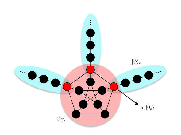
∣ψ⟩=∣ψ⟩G+v∑∣ψ⟩v−v∑av∣0v⟩ where ∣ψ⟩G=∑v∈V∣v⟩⟨v∣ψ⟩ (note in our definition, ∣v⟩=∣0v⟩), ∣ψ⟩v=∑n=0∞∣nv⟩⟨nv∣ψ⟩ and av=⟨0v∣ψ⟩G=⟨0v∣ψ⟩v.
To solve the eigen-decomposition problem H∣ψ⟩=E∣ψ⟩, we have
H∣ψ⟩=HG∣ψ⟩G+HGv∑(∣ψ⟩v−av∣0v⟩)+v∑Hv(∣ψ⟩G−v′∑av′∣0v′⟩)+v∑Hv∣ψ⟩v where gray parts are zeroed out.
Let us assume ∣ψ⟩v=Iv∣−k⟩+Rv∣k⟩, we have
av=Iv+Rv. By inserting (2) to (5), we have
H∣ψ⟩=HG∣ψ⟩G+v∑cos(k)∣ψ⟩v−(2Iveik+2Rve−ik)∣0v⟩ For this ansatz, the eigenvalue of H has to be E=cos(k). By using (4) and (6)
=cos(k)(∣ψ⟩G+v∑∣ψ⟩v−v∑(Iv+Rv)∣0v⟩)HG∣ψ⟩G+v∑cos(k)∣ψ⟩v−v∑(2Iveik+2Rve−ik)∣0v⟩ That is
HG∣ψ⟩G==cos(k)∣ψ⟩G+v∑(−cos(k)(Iv+Rv)+2Iveik+2Rve−ik)∣0v⟩cos(k)∣ψ⟩G−v∑(2Ive−ik+2Rveik)∣0v⟩ Let us assume the scattering is from vertex w, i.e. Iw=1 and Iv=w=0. We have
HG∣ψ⟩G=cos(k)∣ψ⟩G−21e−ik∣0w⟩−v∑2Rveik∣0v⟩ Let z=eik, we have
2HGz∣ψ⟩G=(1+z2)∣ψ⟩G−∣0w⟩−v∑Rvz2∣0v⟩(1−2HGz+Qz2)∣ψ⟩G=(1−z2)∣0w⟩ where
Q=1−v∑∣0v⟩⟨0v∣ since
av=⟨0v∣ψ⟩G={Rv1+Rw,v=w,v=w Except the −2 before HG due to the difference in convension, (11) is the same as Eq. 12 in Ref. 1.
There are two types of bound states. The first type with ∣ψ⟩v=0 is trivial. In the following, we discuss the second type: k=iκ is pure imaginary. Let us assume
∣ψ⟩v=av∣κ⟩ with ∣κ⟩=e−κnv∣nv⟩. Following the same derivation from (7) to (11), we have
H∣ψ⟩=HG∣ψ⟩G+v∑cosh(κ)∣ψ⟩v−2aveκ∣0v⟩ For this ansatz, the eigenvalue of H has to be E=cosh(κ). By using (4) and (14)
=cosh(κ)(∣ψ⟩G+v∑∣ψ⟩v−v∑av∣0v⟩)HG∣ψ⟩G+v∑cosh(κ)∣ψ⟩v−v∑2aveκ∣0v⟩,HG∣ψ⟩G=cosh(κ)∣ψ⟩G−v∑2ave−κ∣0v⟩ Let zb=e−κ, we have a new quadratic linear equation for the bounded states
(1−2HGzb+Qzb2)∣ψ⟩G=0