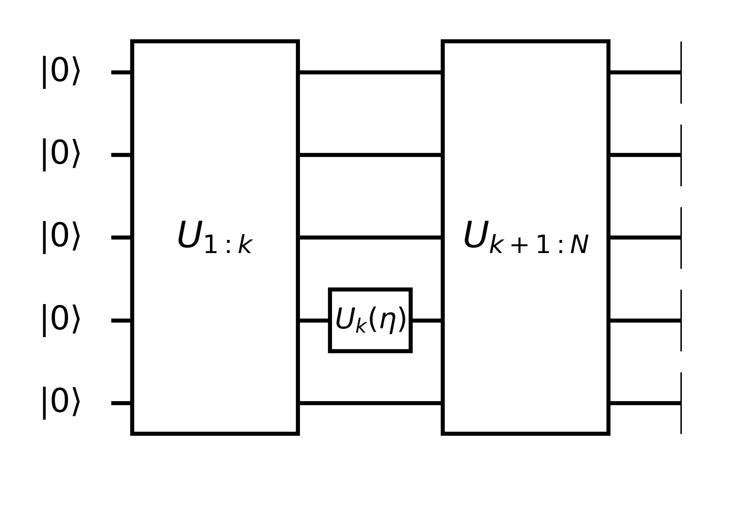
This section is a simplified discussion of results in Ref. 5.
Consider the expectation value of B on state ∣ψN⟩=UN:k+1Uk(η)Uk−1:1∣ψ0⟩ with Uk(η)=e−iΞη/2. Given Ξ2=1, we have Uk(η)=cos(2η)−isin(2η)Ξ.
⟨B⟩=⟨ψk∣[cos2η+isin2ηΞ]B~k+1[cos2η−isin2ηΞ]∣ψk⟩=cos22η⟨ψk∣B~k+1∣ψk⟩+sin22η⟨ψk∣ΞB~k+1Ξ∣ψk⟩+isin2ηcos2η⟨ψk∣[Ξ,B~k+1]∣ψk⟩=cos22η(⟨ψk∣B~k+1−ΞB~k+1Ξ∣ψk⟩)+i2sinη⟨ψk∣[Ξ,B~k+1]∣ψk⟩+⟨ψk∣ΞB~k+1Ξ∣ψk⟩=2cosη(⟨ψk∣B~k+1−ΞB~k+1Ξ∣ψk⟩)+i2sinη⟨ψk∣[Ξ,B~k+1]∣ψk⟩+21⟨ψk∣B~+ΞB~k+1Ξ∣ψk⟩=αcosη+βsinη+γ=rcos(η−ϕ)+γ Here, In line 1, we used the following shorthands
∣ψk⟩=Uk:1∣ψ0⟩B~k+1=UN:k+1†BUN:k+1 And in line 5, we have introduced
αβγ=21(⟨ψk∣B~k+1−ΞB~k+1Ξ∣ψk⟩),=i21⟨ψk∣[Ξ,B~k+1]∣ψk⟩,=21⟨ψk∣B~+ΞB~k+1Ξ∣ψk⟩. Finally, we obtained a sine function.

A direct proposition is
∂η∂⟨B⟩η=21(⟨B⟩η+2π−⟨B⟩η−2π) Next, we describe a new class of differenciable loss which can not be written as an obserable easily, the statistic functionals, for simplicity, we consider an arbitrary statistic functional f(X), with a sequence of bit strings X≡{x1,x2,…,xr} as its arguments. Let's define the following expectation of this function
Ef(Γ)≡{xi∼pθ+γi}i=1rE[f(X)]. Here, Γ={γ1,γ2,…,γr} is the offset angles applied to circuit parameters, %Its element γi is defined in the same parameter space as θ that represents a shift to θ. which means the probability distributions of generated samples is {pθ+γ1,pθ+γ2,…,pθ+γr}. Writing out the above expectation explicitly, we have
Ef(Γ)=X∑f(X)i∏pθ+γi(xi), where index i runs from 1 to r. Its partial derivative with respect to θlα is
∂θlα∂Ef(Γ)=X∑f(X)j∑∂θlα∂pθ+γj(xj)i=j∏pθ+γi(xi) Again, using the gradient of probability, we have
∂θlα∂Ef(Γ)=21j,s=±∑X∑f(X)pθ+γj+s2πelα(xj)i=j∏pθ+γi(xi)=21j,s=±∑Ef({γi+sδij2πelα}i=1r) If f is symmetric, Ef(0) becomes a V-statistic [Mises (1947)], then the gradient can be further simplified to
∂θlα∂Ef(Γ)=2rs=±∑Ef({γ0+s2πelα,γ1,…,γr}), which contains only two terms. This result can be readily verified by calculating the gradient of MMD loss, noticing the expectation of a kernel function is a V-statistic of degree 2. By repeatedly applying the gradient formula, we will be able to obtain higher order gradients.
Jin-Guo Liu and Lei Wang, arXiv:1804.04168
J. Li, X. Yang, X. Peng, and C.-P. Sun, Phys. Rev. Lett. 118,
150503 (2017).
E. Farhi and H. Neven, arXiv:1802.06002.
K. Mitarai, M. Negoro, M. Kitagawa, and K. Fujii,
arXiv:1803.00745.
Nakanishi, Ken M., Keisuke Fujii, and Synge Todo.
arXiv:1903.12166 (2019).
