Complex value networks allows the input/variables in networks being complex, while the loss keeping real. In this post, I will

• derive back propagation formula for complex valued neural network units.

• provide a table of reference for widely used complex neural network units.

Back Propagation for Complex Variables

The gradient for real cost function $J(z)$ defined on complex plane $z=x+iy$ is

In the last line, we have used the reality of $J$. In the following complex version of BP will be derived in order to get $\frac{\partial J}{\partial z}$ layer by layer

Here, $y_l$ and $y_{l+1}$ are variables (including input nodes and network variables) in the $l$-th layer and $l+1$-th layer respectively, and $y_{l+1}=f_l(y_l)$.

• If $f_l$ is holomophic (sometimes called differenciable, entire, maybe different?), we have contributions from the second term vanish, thus

which is the exactly the same BP formula as for real functions except here we take its conjugate.

• If $f_l$ is non-holomophic, we have

Difference made clear: a numerical test

Given input vector $x$ of length $10$, our toy network gives output $J=f_2(f_1(f_1(x)))$ as a cost function, where $f_1(z)=z^*$ and $f_2(z)=-e^{-\vert z\vert^2}$. This is simple function, naive BP like real network will fail. Code is attached at the end of blog.

Result:

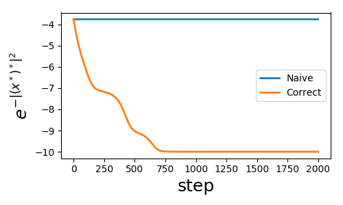
Only the correct fomulation (above notes) converges to $-10$ correctly, the old holomophic version naive realization is incorrect.

A table of reference

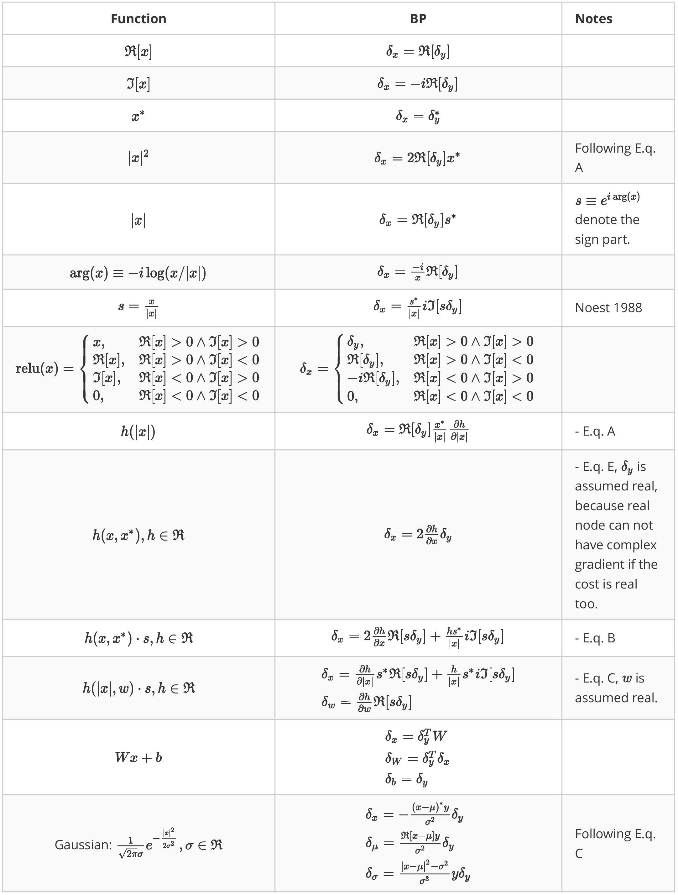
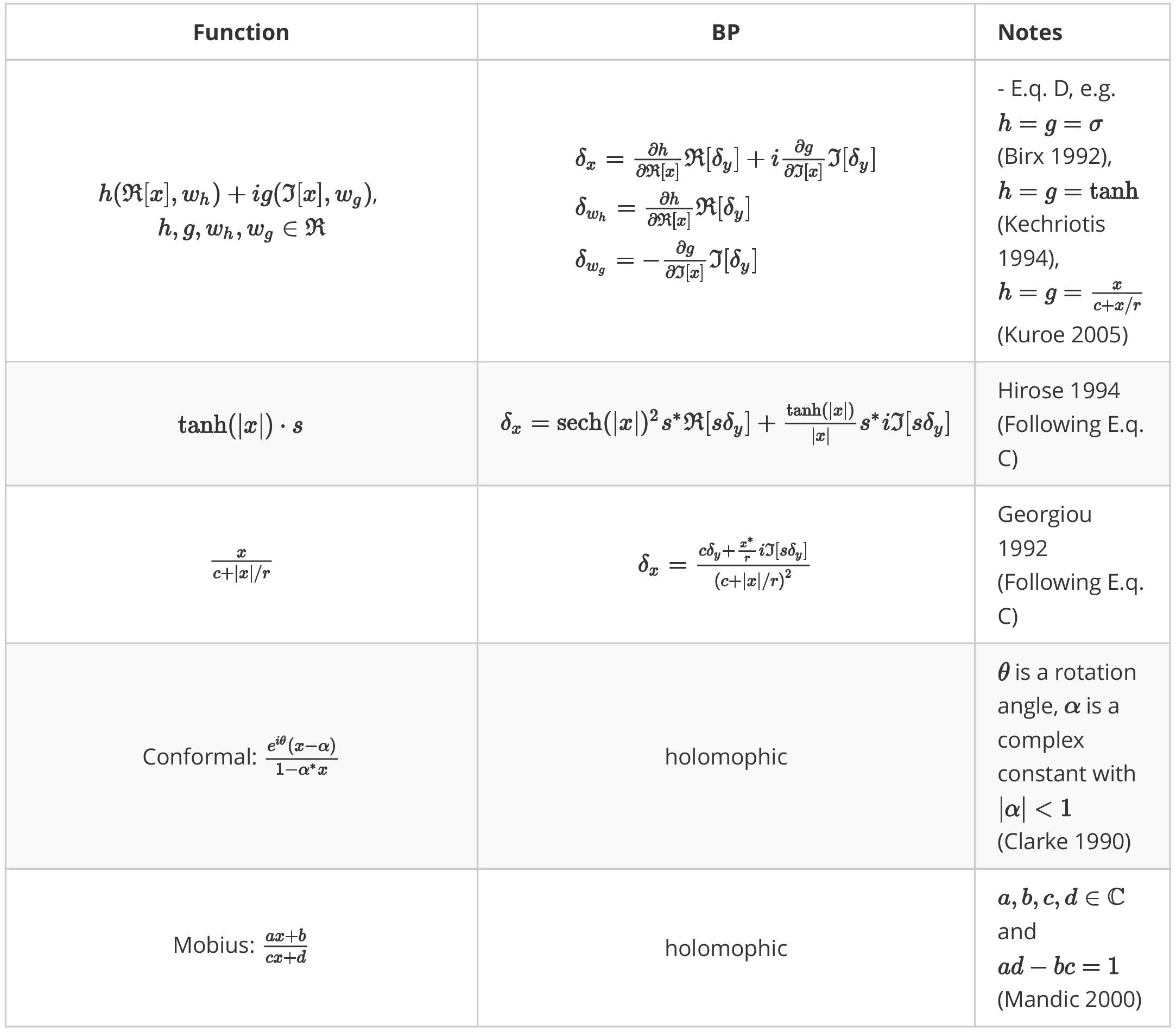
Equation $A, B, C$ are meta functions, each of them generates a class of non-holomophic function.

All these functions are realized checked strictly using numerical differenciation.

If you want to know more or write a library on it

• You can read Akira's "Complex Valued Neural Networks".

• Or just contact me: cacate0129@iphy.ac.cn

Personal views on Complex Valued Networks

holomophic and non-holomophic functions

Many people in computer science states that complex functions can be replaced by double sized real networks, that is not true. This brings us to the old question why complex values are needed? If there is no complex number,

• unitary matrices can not be easily implemented.

• nature of phase can not be neatly represented, light and holograph, sound, quantum wavefunction et. al.

Although a complex valued network must contain at least one non-holomophic function (to make the loss real), I believe the essense of complex valued functions are holomophism. If a function is not holomophic, it will make no big difference with double sized real functions.

Liouville's theorem gives many interesting results on holomophic complex functions

• Every bounded entire function must be constant

• If f is less than or equal to a scalar times its input, then it is linear

• ...

these properties will give us chance and challenge to implement complex valued networks.

Complex networks tend to blow up

These properties usually means they tend to blow up. Which means, we can not define "soft" functions like sigmoid, tanh.

Appendix

Code for back-propagation test

'''
Test complex back propagation.
The theory could be found in Akira's book "Complex Valued Neural Networks".
'''

import numpy as np
from matplotlib.pyplot import *

# define two useful functions and their derivatives.
def f1_forward(x): return x.conj()


def df1_z(x, y): return np.zeros_like(x, dtype='complex128')


def df1_zc(x, y): return np.ones_like(x, dtype='complex128')


def f2_forward(x): return -np.exp(-x * x.conj())


def df2_z(x, y): return -y * x.conj()


def df2_zc(x, y): return -y * x

# we compare the correct and incorrect back propagation
def naive_backward(df_z, df_zc):
    '''
    naive back propagation meta formula,
    df_z and df_zc are dirivatives about variables and variables' conjugate.
    '''
    return lambda x, y, dy: df_z(x, y) * dy


def correct_backward(df_z, df_zc):
    '''the correct version.'''
    return lambda x, y, dy: df_z(x, y) * dy +\
                    df_zc(x, y).conj() * dy.conj()


# the version in naive bp
f1_backward_naive = naive_backward(df1_z, df1_zc)
f2_backward_naive = naive_backward(df2_z, df2_zc)

# the correct backward propagation
f1_backward_correct = correct_backward(df1_z, df1_zc)
f2_backward_correct = correct_backward(df2_z, df2_zc)

# initial parameters, and network parameters
num_input = 10
a0 = np.random.randn(num_input) + 1j * np.random.randn(num_input)
num_layers = 3


def forward(x):
    '''forward pass'''
    yl = [x]
    for i in range(num_layers):
        if i == num_layers - 1:
            x = f2_forward(x)
        else:
            x = f1_forward(x)
        yl.append(x)
    return yl


def backward(yl, version):  # version = 'correct' or 'naive'
    '''
    back propagation, yl is a list of outputs.
    '''
    dy = 1 * np.ones(num_input, dtype='complex128')
    for i in range(num_layers):
        y = yl[num_layers - i]
        x = yl[num_layers - i - 1]
        if i == 0:
            dy = eval('f2_backward_%s' % version)(x, y, dy)
        else:
            dy = eval('f1_backward_%s' % version)(x, y, dy)
    return dy.conj() if version == 'correct' else dy


def optimize_run(version, alpha=0.1):
    '''simple optimization for target loss function.'''
    cost_histo = []
    x = a0.copy()
    num_run = 2000
    for i in range(num_run):
        yl = forward(x)
        g_a = backward(yl, version)
        x[:num_input] = (x - alpha * g_a)[:num_input]
        cost_histo.append(yl[-1].sum().real)
    return np.array(cost_histo)


if __name__ == '__main__':
    lr = 0.01
    cost_r = optimize_run('naive', lr)
    cost_a = optimize_run('correct', lr)
    figure(figsize=(5,3))
    plot(cost_r, lw=2)
    plot(cost_a, lw=2)
    legend(['Naive', 'Correct'])
    ylabel(r'$e^{-|(x^*)^*|^2}$', fontsize = 18)
    xlabel('step', fontsize = 18)
    tight_layout()
    show()